The concept of conditional probability is a useful one. There are countless real world examples where the probability of one event is conditional on the probability of a previous one. While the sum and product rules of probability theory can anticipate this factor of conditionality, in many cases such calculations are NP-hard. The prospect of managing a scenario with 5 discrete random variables (25-1=31 discrete parameters) might be manageable. An expert system for monitoring patients with 37 variables resulting in a joint distribution of over 237 parameters would not be manageable[6] [1].
Consider a domain U of n variables, x1,...xn. Each variable may be discrete having a finite or countable number of states, or continuous. Given a subset X of variables xi where xi ![]() U, if one can observe the state of every variable in X, then this observation is called an instance of X and is denoted as X=
U, if one can observe the state of every variable in X, then this observation is called an instance of X and is denoted as X=![]()
![]() for the observations
for the observations ![]() . The "joint space" of U is the set of all instances of U.
. The "joint space" of U is the set of all instances of U. ![]() denotes the "generalized probability density" that X=
denotes the "generalized probability density" that X=![]()
![]() given Y=
given Y=![]() for a person with current state information
for a person with current state information ![]() . p(X|Y,
. p(X|Y, ![]() ) then denotes the "Generalized Probability Density Function" (gpdf) for X, given all possible observations of Y. The joint gpdf over U is the gpdf for U.
) then denotes the "Generalized Probability Density Function" (gpdf) for X, given all possible observations of Y. The joint gpdf over U is the gpdf for U.
A Bayesian network for domain U represents a joint gpdf over U. This representation consists of a set of local conditional gpdfs combined with a set of conditional independence assertions that allow the construction of a global gpdf from the local gpdfs. As shown previously, the chain rule of probability can be used to ascertain these values:
One assumption imposed by Bayesian Network theory (and indirectly by the Product Rule of probability theory) is that each variable xi, ![]() must be a set of variables that renders xi and {x1,...xi-1} conditionally independent. In this way:
must be a set of variables that renders xi and {x1,...xi-1} conditionally independent. In this way:
A Bayesian Network Structure then encodes the assertions of conditional independence in equation 10 above. Essentially then, a Bayesian Network Structure Bs "is a directed acyclic graph such that (1) each variable in U corresponds to a node in Bs, and (2) the parents of the node corresponding to xi are the nodes corresponding to the variables in [Pi]i."[8] [3]
"A Bayesian-network gpdf set Bp is the collection of local gpdfs ![]() for each node in the domain."[9] [4]
for each node in the domain."[9] [4]
Given a situation where it might rain today, and might rain tomorrow, what is the probability that it will rain on both days? Rain on two consecutive days are not independent events with isolated probabilities. If it rains on one day, it is more likely to rain the next. Solving such a problem involves determining the chances that it will rain today, and then determining the chance that it will rain tomorrow conditional on the probability that it will rain today. These are known as "joint probabilities." Suppose that P(rain today) = 0.20 and P(rain tomorrow given that it rains today) = 0.70. The probability of such joint events is determined by:
 (eq. 12)
which can also be expressed as:
 (eq. 13)[10] [5]
Working out the joint probabilities for all eventualities, the results can be expressed in a table format:
| Rain Tomorrow | No Rain Tomorrow | Marginal Probability of Rain Today | |
|---|---|---|---|
| Rain Today | 0.14 | 0.06 | 0.20 |
| No Rain Today | 0.16 | 0.64 | 0.80 |
| Marginal Probability of Rain Tomorrow | 0.30 | 0.70 |
From the table, it is evident that the joint probability of rain over both days is 0.14, but there is a great deal of other information that had to be brought into the calculations before such a determination was possible. With only two discrete, binary variables, four calculations were required.
This same scenario can be expressed using a Bayesian Network Diagram as shown ("!" is used to denote "not").
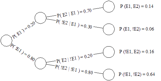
Figure 1: A Bayesian Network showing the probability of rain
One attraction of Bayesian Networks is the efficiency that only one branch of the tree needs to be traversed. We are really only concerned with P(E1), P(E2|E1) and P(E2,E1).
We can also utilize the graph both visually and algorithmically to determine which parameters are independent of each other. Instead of calculating four joint probabilities, we can use the independence of the parameters to limit our calculations to two. It is self-evident that the probabilities of rain on the second day having rained on the first are completely autonomous from the probabilities of rain on the second day having not rained on the first.
At the same time as emphasizing parametric indifference, Bayesian Networks also provide a parsimonious representation of conditionality among parametric relationships. While the probability of rain today and the probability of rain tomorrow are two discrete events (it cannot rain both today and tomorrow at the same time), there is a conditional relationship between them (if it rains today, the lingering weather systems and residual moisture are more likely to result in rain tomorrow). For this reason, the directed edges of the graph are connected to show this dependency.
Friedman and Goldszmidt suggest looking at Bayesian Networks as a "story". They offer the example of a story containing five random variables: "Burglary", "Earthquake", "Alarm", "Neighbour Call", and "Radio Announcement".[11] [6] In such a story, "Burglary" and "Earthquake" are independent, and "Burglary" and "Radio Announcement" are independent given "Earthquake." This is to say that there is no event which effects both burglaries and earthquakes. As well, "Burglary" and "Radio Announcements" are independent given "Earthquake"--meaning that while a radio announcement might result from an earthquake, it will not result as a repercussion from a burglary.
Because of the independence among these variables, the probability of P(A,R,E,B) (The joint probability of an alarm, radio announcement, earthquake and burglary) can be reduced from:
P(A,R,E,B)=P(A|R,E,B)*P(R|E,B)*P(E|B)*P(B)
involving 15 parameters to 8:
P(A,R,E,B) = P(A|E,B)*P(R|E)*P(E)*P(B)
This significantly reduced the number of joint probabilities involved. This can be represented as a Bayesian Network:
![--[The conditional probabilities of an alarm giving the independent events of a burglary and earthquake]--](/sites/default/files/bayes35.gif)
Figure 2: The conditional probabilities of an alarm given the independent events of a burglary and earthquake.
Using a Bayesian Network offers many advantages over traditional methods of determining causal relationships. Independence among variables is easy to recognize and isolate while conditional relationships are clearly delimited by a directed graph edge: two variables are independent if all the paths between them are blocked (given the edges are directional). Not all the joint probabilities need to be calculated to make a decision; extraneous branches and relationships can be ignored (One can make a prediction of a radio announcement regardless of whether an alarm sounds). By optimizing the graph, every node can be shown to have at most k parents. The algorithmic routines required can then be run in O(2kn) instead of O(2n) time. In essence, the algorithm can run in linear time (based on the number of edges) instead of exponential time (based on the number of parameters).[12] [7]
Associated with each node is a set of conditional probability distributions. For example, the "Alarm" node might have the following probability distribution:[13] [8]
| E | B | P(A | E,B) | P(!A|E,B) |
|---|---|---|---|
| E | B | 0.90 | 0.10 |
| E | !B | 0.20 | 0.80 |
| !E | B | 0.90 | 0.10 |
| !E | !B | 0.01 | 0.99 |
For example, should there be both an earthquake and a burglary, the alarm has a 90% chance of sounding. With only an earthquake and no burglary, it would only sound in 20% of the cases. A burglary unaccompanied by an earthquake would set off the alarm 90% of the time, and the chance of a false alarm given no antecedent event should only have a probability of 0.1% of the time. Obviously, these values would have to be determined a posteriori.
Links
[1] https://niedermayer.ca/node/31#fn5
[2] https://niedermayer.ca/node/31#fn6
[3] https://niedermayer.ca/node/31#fn7
[4] https://niedermayer.ca/node/31#fn8
[5] https://niedermayer.ca/node/31#fn9
[6] https://niedermayer.ca/node/31#fn10
[7] https://niedermayer.ca/node/31#fn11
[8] https://niedermayer.ca/node/31#fn12